Deep-learning ASR convolutional-neural-networks
In this post we are going to see an example of CNN (convolutional neural networks) applied to speech recognition application.
The goal of our machine learning model based on CNN’s Deep Learning algorithms will be to classify some simple words, starting with numbers from zero to nine.
To extract the distinctive features of speech, we will first adopt a voice coding procedure rather used in the ASR area (Automatic Speech Recognition) named Mel Frequency Cepstral Coefficient or more simply MFCC.
Thanks to the MFCC technique we will be able to encode every single word spoken vocally into a sequence of vectors, each of them 13 value-long representing the MFCC algorithm coefficients.
In our case – being the single words represented by single-digit numbers – we will go to encode each single number by using a 48 x 13 matrix.

The previous image shows the chain of the main modules involved during an MFCC encoding process: the voice signal is segmented into several frames of proper duration in the time domain (generally 25-40 ms).
For each of these segments we are going to calculate the the power spectrum densityThe result is provided as input to a series of partially overlapping filters (filter bank) which calculate the spectral density of energy corresponding to different frequency ranges of our power spectrum.
26 coefficients are obtained for each frame, made by the result of the energy spectrum downstream of each filter. The result is finally processed through the discrete cosine transform or DCT (Discrete Cosine Transform).
DCT has the property of being able to encode the signal features by using the low frequencies as best as possibile: a useful feature since we are dealing with a voice signal, whose main properties are between 300 and 3400 Hz give or take a few.
Final result: at the end of this process, the MFCC provides us with 13 useful coefficients that we will use with proper machine learning algorithms, by deploying some optimal classifiers (in this example based on CNN).
As far as the training phase is concerned, we will use the dataset available here named Free Spoken Digit Dataset: it is about 2000 voice recordings performed with different people who have pronounced the numbers from zero to nine according to different environment and time.
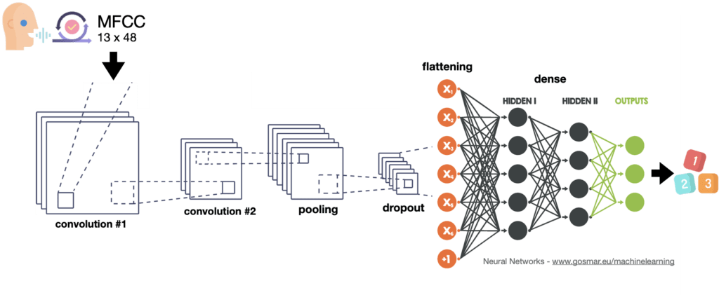
For our classifier we will use the convolutional neural network with different levels here below depicted:
Let’s now see some code and performances!
We can import some useful libraries into our Python Jupyter Notebook:
import pandas as pd
from sklearn.model_selection import train_test_split
import pickle
import matplotlib.pyplot as plt
import matplotlib.ticker as ticker
from IPython.display import HTML
import numpy as np
from sklearn import preprocessing
import matplotlib.pyplot as plt
from scipy.io import wavfile as wav
import scipy
from python_speech_features import mfcc
from python_speech_features import logfbank
import tensorflow as tf
from keras.models import Sequential
from keras.layers import Dense, Flatten, Activation, Dropout, LSTM
from keras.layers import Conv2D, MaxPooling2D, GlobalMaxPooling2D
from keras.optimizers import SGD
import os
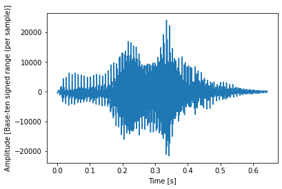
Let’s analyze one of the random voice messages, for example the “0_jackson_0.wav” file:
(rate,sig1) = wav.read(“/Users/diego/Diego/Xenialab/AI/jupyter/digits/0_jackson_0.wav”)
N = sig1.shape[0]
L = N / rate
f, ax = plt.subplots()
ax.plot(np.arange(N) / rate, sig1)
ax.set_xlabel(‘Time [s]’)
ax.set_ylabel(‘Amplitude [Base-ten signed range (per sample)]’);
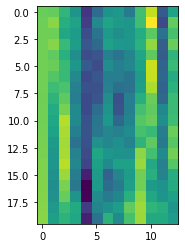
Let’s now see the result of applying the MFCC function to the signal out of curiosity:
mfcc_feat = mfcc(sig1,rate,nfft=512)
plt.imshow(mfcc_feat[0:20,:])
We can also visualize a sort of spectrogram: actually it’s about the 13 outputs of the DCT for each time frame of the signal … here we can see the first twenty.
Likewise, we may have some fun by viewing other signals and several pronunciations!
It’s now time we started doing things seriously.
First of all we are going to import the 2000 voice recording files into a special list of vectors, which we then convert and separate appropriately, thus to obtain the useful values for learning and the target label to predict:
soundfile = os.listdir(‘/Users/diego/Diego/Xenialab/AI/jupyter/digits’)
data=[]
for i in soundfile:
(rate,sig) = wav.read(‘/Users/diego/Diego/Xenialab/AI/jupyter/digits/’+i)
data.append(sig)
#set the independent var
size = 48
X=[]
for i in range(len(data)):
mfcc_feat = mfcc(data[i],rate,nfft=512)
mfcc_feat = np.resize(mfcc_feat, (size,13))
X.append(mfcc_feat)
X = np.array(X)
#set the target label
y = [i[0] for i in soundfile]
Y = pd.get_dummies(y)
The target label is nothing more than a matrix values “1” for each of the 2000 recorded files according to the pronounced number.
Let’s see the first three lines of this matrix:
print(Y[0:3])
   0  1  2  3  4  5  6  7  8  9
0  0  0  0  0  0  1  0  0  0  0
1  0  0  0  1  0  0  0  0  0  0
2  0  0  0  0  1  0  0  0  0  0
So the first three loaded recordings correspond to the numbers five, three and four.
Let’s convert the target label into a suitable matrix:
Y = np.array(Y)
We may also print the format of the independent variable X to better understand:
print(X.shape)
(2000, 48, 13)
Therefore, X is composed of 2000 48 x 13 matrices corresponding to the features extracted with the MFCC function for each voice recording.
It’s now time to carry out the learning process by using the convolutional neural network. Let’s have a look at it again:

This type of architecture can also be used for many other applications, including image recognition and several kind of classifications. In this case let’s apply it to reach our goal: voice recognition.
model = Sequential()
#Convolution layers
model.add(Conv2D(8, (3, 3), activation=’relu’, input_shape=(size, 13,1)))
model.add(Conv2D(8, (3, 3), activation=’relu’))
model.add(MaxPooling2D(pool_size=(2, 2)))
model.add(Dropout(0.1))
#Flattening
model.add(Flatten(input_shape=(size, 13,1)))
#1st fully connected Neural Network hidden-layer
model.add(Dense(64))
model.add(Dropout(0.16))
model.add(Activation(‘relu’))
#2nd fully connected Neural Network hidden-layer
model.add(Dense(64))
model.add(Dropout(0.12))
model.add(Activation(‘relu’))
#Output layer
model.add(Dense(10))
model.add(Activation(‘softmax’))
model.summary()
Model: "sequential_1"
_________________________________________________________________
Layer (type)                 Output Shape              Param #
=================================================================
conv2d_1 (Conv2D)            (None, 46, 11, 8)         80
_________________________________________________________________
conv2d_2 (Conv2D)            (None, 44, 9, 8)          584
_________________________________________________________________
max_pooling2d_1 (MaxPooling2 (None, 22, 4, 8)          0
_________________________________________________________________
dropout_1 (Dropout)          (None, 22, 4, 8)          0
_________________________________________________________________
flatten_1 (Flatten)          (None, 704)               0
_________________________________________________________________
dense_1 (Dense)              (None, 64)                45120
_________________________________________________________________
dropout_2 (Dropout)          (None, 64)                0
_________________________________________________________________
activation_1 (Activation)    (None, 64)                0
_________________________________________________________________
dense_2 (Dense)              (None, 64)                4160
_________________________________________________________________
dropout_3 (Dropout)          (None, 64)                0
_________________________________________________________________
activation_2 (Activation)    (None, 64)                0
_________________________________________________________________
dense_3 (Dense)              (None, 10)                650
_________________________________________________________________
activation_3 (Activation)    (None, 10)                0
=================================================================
Total params: 50,594
Trainable params: 50,594
Non-trainable params: 0
Let’s now compile the model by using the SGD optimizer:
sgd = SGD(lr=0.01, decay=1e-6, momentum=0.9, nesterov=True)
model.compile(loss=’binary_crossentropy’,
optimizer=sgd,
metrics=[‘accuracy’])
We need to separate the training and test data and make them of the proper size to be recognized as proper tensors by our CNN network:
x_train, x_test, y_train, y_test = train_test_split(X, Y, test_size=0.25)
x_train = x_train.reshape(-1, size, 13, 1)
x_test = x_test.reshape(-1, size, 13, 1)
Let’s fit the model and evaluate the performances:
history = model.fit(
x_train,
y_train,
epochs=18,
batch_size=32,
validation_split=0.2,
shuffle=True
)
model.evaluate(x_test, y_test, verbose=2)
Train on 1200 samples, validate on 300 samples
Epoch 1/18
1200/1200 [==============================] - 1s 469us/step - loss: 0.3319 - accuracy: 0.8967 - val_loss: 0.2683 - val_accuracy: 0.9070
Epoch 2/18
1200/1200 [==============================] - 0s 256us/step - loss: 0.2534 - accuracy: 0.9066 - val_loss: 0.1943 - val_accuracy: 0.9217
...
...
Epoch 18/18 1200/1200 [==============================] - 0s 254us/step - loss: 0.0444 - accuracy: 0.9837 - val_loss: 0.0425 - val_accuracy: 0.9880
Out[24]:
[0.039418088585138324, 0.9860000610351562]
Here are the cost function (loss) and accuracy:
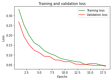
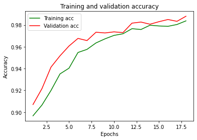
Conclusions: not bad at all!
We had to work a little bit on CNN’s various parameters to get such results.
Let’s try the inference by predicting one of the recorded messages available inside the test dataset.
#Print the sound to be predicted
sound_index = 10
y_test[sound_index]
array([0, 0, 0, 0, 0, 0, 1, 0, 0, 0], dtype=uint8)
It is in this case the number is six.
Here is the prediction made with by using our model:
pred = model.predict(x_test[sound_index].reshape(-1,size,13,1))
print(“\n\033[1mPredicted digit sound: %.0f”%pred.argmax(),”\033[0m \n “)
print(“Predicted probability array:”)
print(pred)
Predicted digit sound: 6

Predicted probability array:
[[3.8950305e-02 9.8831032e-04 7.7098295e-02 8.1201904e-02 2.2223364e-03
  4.8808311e-04 6.2295502e-01 1.0375674e-03 1.6901042e-01 6.0477410e-03]]
Our artificial intelligence neural model designed for speech recognition was able to predict the value six correctly with probability equal 0.623.
The second closest value to this prediction is the number eight, with a probability of approximately 0.169.
Obviously to better refine our code we will save the learning model (for example on a disk) and then use it online during the prediction phase: it must be near real time to fit with a speech recognition application.
Do you want to know more about this techniques?
Here is an interesting book on Machine Learning and AI.
https://www.amazon.com/dp/B08GFL6NVM
