We described in one of the previous posts how to use convolutional neural networks, in order to perform speech recognition related to simple numbers from zero to nine.
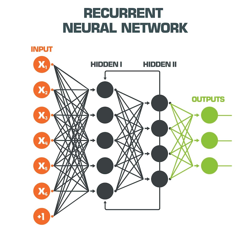
In practice, speech recognition has superior performance by adopting particular neural networks called Recurrent Neural Networks, or simply RNNs.
Unlike “simple” feed-forward neural networks, RNNs process as input both the data currently provided as such, plus some of the output data provided retroactively. This allows them to work “with memory“.
Among the RNN recurrent neural networks offering better performance when we want to make predictions that require memory, or take into account the sequence of previous incoming data, we can include the type called LSTM, or Long short-term memory. They are able to predict the outputs taking into account even very antecedent data, that is, we could say that “they have a long memory“.
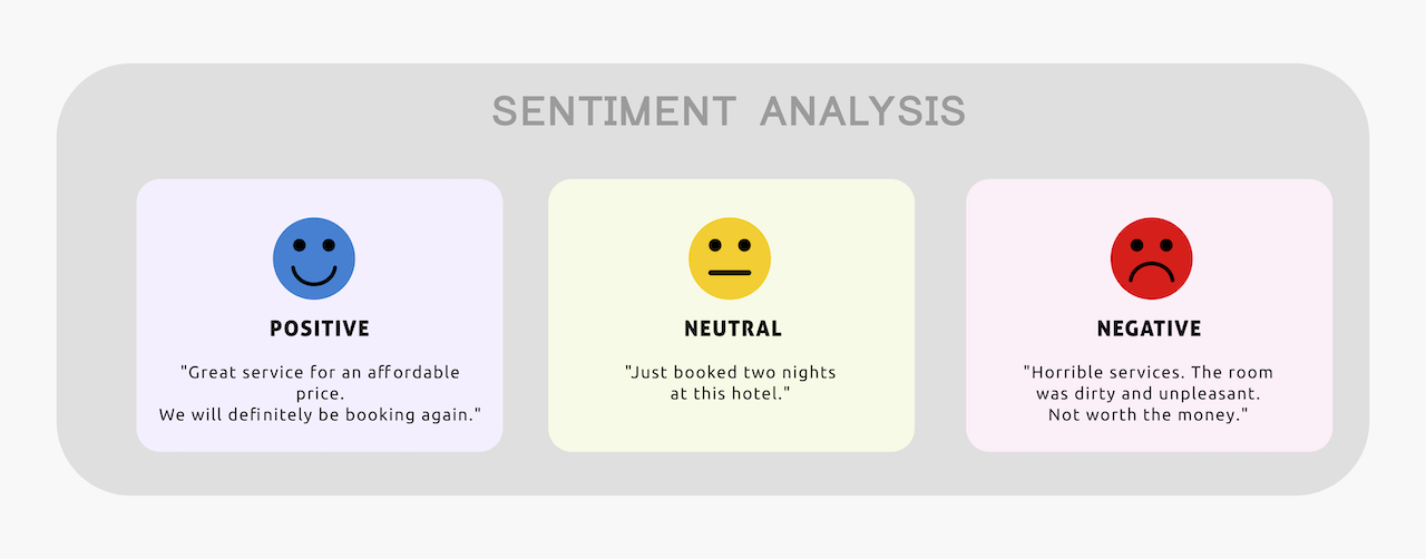
In the following post, we will use the LSTMs to carry out a Sentiment analysis on some data. In particular, we will import a public dataset of reviews of 25,000 films, available to train and validate our machine learning model with neural network design using LSTM methodologies.
A similar model could be used to carry out speech analysis, i.e. analysis of the contents of voice messages and conversations of various types, in order to extract features and predict sentiment or other useful characteristics according to the context of interest (i.e political and social interests or buying preferences for brands etc …).
Let’s import the necessary libraries, including the entire Keras suite to design and train the recurrent neural network:
import pandas as pd
from sklearn.model_selection import train_test_split
import pickle
import matplotlib.pyplot as plt
import matplotlib.ticker as ticker
from IPython.display import HTML
import numpy as np
from sklearn import preprocessing
from keras.datasets import imdb
from keras.models import Sequential
from keras.preprocessing.sequence import pad_sequences
from keras.layers import Embedding, GlobalAveragePooling1D, Dense, SpatialDropout1D, LSTM, Dropout
from keras.optimizers import SGD
from keras.preprocessing.text import Tokenizer
from keras.utils import to_categorical
Let’s set the maximum number of words we will use in our dictionary and the maximum length of each review:
# Define max dictionary words and max lenght of each review
num_words = 12000
max_phrase_len = 256
Let’s then import the IMDB dataset provided by Keras:
# Import the IMDB movie reviews
(X_train, y_train), (X_test, y_test) = imdb.load_data(num_words=num_words)
# Display number of training and testing data
print(“Training entries: {}, labels: {}”.format(len(X_train), len(y_train)))
More information on the IMDB dataset is available on the official website:
https://keras.io/api/datasets/imdb/
As described, the dataset contains 25,000 reviews of various English-language films. Each word in the review has already been converted to an integer. For convenience, this conversion took place using the frequency of the word within the dataset: for example, the word “worst” is converted with the number 249 precisely because it appears 249 times in the dataset under examination.
This process (as we will illustrate later) spare us the task of text tokenization otherwise indispensable.
Let’s insert an offset equal to 3, in order to add and associate the values 0,1,2,3 respectively to the PAD label (useful for “filling” reviews with a length of less than 256), START, UNKNOWN and UNUSED:
INDEX_FROM=3
word_to_id = imdb.get_word_index()
word_to_id = {k:(v+INDEX_FROM) for k,v in word_to_id.items()}
word_to_id[“<PAD>”] = 0
word_to_id[“<START>”] = 1
word_to_id[“<UNK>”] = 2
word_to_id[“<UNUSED>”] = 3
id_to_word = {value:key for key,value in word_to_id.items()}
Let’s see an example of a positive review both in numerical and textual format (the first of the reviews of the training set):
# Positive review example
print(X_train[0])
print(‘ ‘.join(id_to_word[id] for id in X_train[0] ))
[1, 14, 22, 16, 43, 530, 973, 1622, 1385, 65, 458, 4468, 66, 3941, 4, 173, 36, 256, 5, 25, 100, 43, 838, 112, 50, 670, 2, 9, 35, 480, 284, 5, 150, 4, 172, 112, 167, 2, 336, 385, 39, 4, 172, 4536, 1111, 17, 546, 38, 13, 447, 4, 192, 50, 16, 6, 147, 2025, 19, 14, 22, 4, 1920, 4613, 469, 4, 22, 71, 87, 12, 16, 43, 530, 38, 76, 15, 13, 1247, 4, 22, 17, 515, 17, 12, 16, 626, 18, 2, 5, 62, 386, 12, 8, 316, 8, 106, 5, 4, 2223, 5244, 16, 480, 66, 3785, 33, 4, 130, 12, 16, 38, 619, 5, 25, 124, 51, 36, 135, 48, 25, 1415, 33, 6, 22, 12, 215, 28, 77, 52, 5, 14, 407, 16, 82, 10311, 8, 4, 107, 117, 5952, 15, 256, 4, 2, 7, 3766, 5, 723, 36, 71, 43, 530, 476, 26, 400, 317, 46, 7, 4, 2, 1029, 13, 104, 88, 4, 381, 15, 297, 98, 32, 2071, 56, 26, 141, 6, 194, 7486, 18, 4, 226, 22, 21, 134, 476, 26, 480, 5, 144, 30, 5535, 18, 51, 36, 28, 224, 92, 25, 104, 4, 226, 65, 16, 38, 1334, 88, 12, 16, 283, 5, 16, 4472, 113, 103, 32, 15, 16, 5345, 19, 178, 32]
<START> this film was just brilliant casting location scenery story direction everyone's really suited the part they played and you could just imagine being there robert <UNK> is an amazing actor and now the same being director <UNK> father came from the same scottish island as myself so i loved the fact there was a real connection with this film the witty remarks throughout the film were great it was just brilliant so much that i bought the film as soon as it was released for <UNK> and would recommend it to everyone to watch and the fly fishing was amazing really cried at the end it was so sad and you know what they say if you cry at a film it must have been good and this definitely was also congratulations to the two little boy's that played the <UNK> of norman and paul they were just brilliant children are often left out of the <UNK> list i think because the stars that play them all grown up are such a big profile for the whole film but these children are amazing and should be praised for what they have done don't you think the whole story was so lovely because it was true and was someone's life after all that was shared with us all
Being positive, the target label value will be equal to 1:
# Display the target label
# 0 = negative, 1 = positive
print(y_train[0])
Result: 1
The second review in the training data is negative: you can repeat the previous instructions with X_train [1] and y_train [1] and you will get a result equal to zero.
We can now insert the PAD label, in order to align the length of all reviews to 256, using the pad_sequences function provided by Keras:
#Align the lenght of each training and test review to 256 by adding PAD words
X_train = pad_sequences(
X_train,
value=word_to_id[“”],
padding=’post’,
maxlen=max_phrase_len
)
X_test = pad_sequences(
X_test,
value=word_to_id[“”],
padding=’post’,
maxlen=max_phrase_len
)
Let’s print a review, for example the second one, to view the added PADs:
#Display the result after the Padding process (words)
print(‘ ‘.join(id_to_word[id] for id in X_train[1] ))
<START> big hair big boobs bad music and a giant safety pin these are the words to best describe this terrible movie i love cheesy horror movies and i've seen hundreds but this had got to be on of the worst ever made the plot is paper thin and ridiculous the acting is an abomination the script is completely laughable the best is the end showdown with the cop and how he worked out who the killer is it's just so damn terribly written the clothes are sickening and funny in equal measures the hair is big lots of boobs bounce men wear those cut <UNK> shirts that show off their <UNK> sickening that men actually wore them and the music is just <UNK> trash that plays over and over again in almost every scene there is trashy music boobs and <UNK> taking away bodies and the gym still doesn't close for <UNK> all joking aside this is a truly bad film whose only charm is to look back on the disaster that was the 80's and have a good old laugh at how bad everything was back then <PAD> <PAD> <PAD> <PAD> <PAD> <PAD> <PAD> <PAD> <PAD> <PAD> <PAD> <PAD> <PAD> <PAD> <PAD> <PAD> <PAD> <PAD> <PAD> <PAD> <PAD> <PAD> <PAD> <PAD> <PAD> <PAD> <PAD> <PAD> <PAD> <PAD> <PAD> <PAD> <PAD> <PAD> <PAD> <PAD> <PAD> <PAD> <PAD> <PAD> <PAD> <PAD> <PAD> <PAD> <PAD> <PAD> <PAD> <PAD> <PAD> <PAD> <PAD> <PAD> <PAD> <PAD> <PAD> <PAD> <PAD> <PAD> <PAD> <PAD> <PAD> <PAD> <PAD> <PAD> <PAD> <PAD> <PAD>
Now that we have all the reviews of equal length, we need to transform each word from the associated integer to a set of features that are more suitable to be fed into our neural network-based machine learning model. In fact, if we fed the whole numbers as they are, the model would certainly be subject to high biases because it would associate the numbers with ordinal quantities, without taking into account their textual meaning and correlations.
In order to do this, Keras provides the function called Embedding, which allows you to transform each word (integer) into a multidimensional vector that has a meaning: to simplify, we can think that the more two words are related to each other, the more the embedding function will associate them with two vectors “close” to each other.
Let’s try to print the vectors related to our dataset on a graph, by using the simplest possible embedding function, that is, of two dimensions.
# Evaluate the Embedding operation
model = Sequential()
model.add(Embedding(input_dim=num_words, output_dim=2, input_length=256))
textvector = model.layers[0].get_weights()[0]
# Display the 2D map of word vectorization after the embedding process
x_vect = textvector[:,0]
y_vect = textvector[:,1]
fig = plt.figure()
fig.subplots_adjust(top=3.8, right = 1.9)
ax1 = fig.add_subplot(211)
plt.scatter(x_vect, y_vect, alpha=0.2,c=’pink’) # Plot the vectorized words
plt.scatter(x_vect[2], y_vect[2], alpha=1.0,c=’blue’) # Plot vector for word in position 2
plt.scatter(x_vect[3], y_vect[3], alpha=1.0,c=’blue’) # Plot vector for word in position 2
plt.title(“Word Vectorization”, fontsize=20)
plt.xlabel(“X vector value”, fontsize=20)
plt.ylabel(“Y vector value”, fontsize=20)
Here is the result:
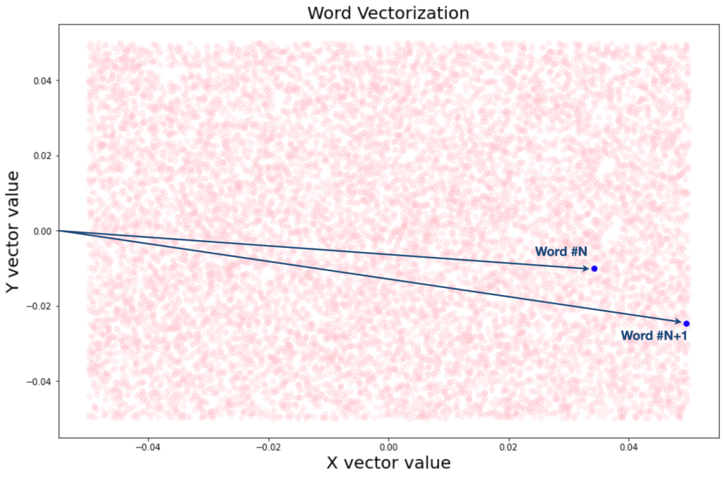
In practice, we will use a 32-dimensional vector space in the embedding next design related to the actual neural network.
The time has come to “draw” our recurrent neural network with Keras. Let’s do it!
# Create the RNN Neural Network
model_lstm = Sequential()
model_lstm.add(Embedding(input_dim = num_words, output_dim = 32, input_length = max_phrase_len))
model_lstm.add(SpatialDropout1D(0.1))
model_lstm.add(LSTM(32, dropout = 0.2, recurrent_dropout = 0.2,return_sequences=True))
model_lstm.add(LSTM(32))
model_lstm.add(Dense(128, activation = ‘relu’))
model_lstm.add(Dropout(0.3))
model_lstm.add(Dense(2, activation = ‘softmax’))
model_lstm.summary()
Our network is therefore made up of an input layer taking care of implementing vectorization through 32-dimensional embedding, thus producing 32 features for each word of the reviews, a second LSTM recurring network layer with long memory (return_sequences = True) and a third with shorter memory (both with 32 nodes).

Then there is a fourth level of fully-connected neural network with 128 nodes and an output level that will provide us with two values: the probability that the review is positive (1) or negative (0).
Obviously, some dimensionality reduction functions are also applied, through different dropouts, in order to refine the model.
Let’s compile in the model:
#Compile the RNN model
model_lstm.compile(
loss=’sparse_categorical_crossentropy’,
optimizer=’Adam’,
metrics=[‘accuracy’]
)
Finally, we can fit the model by passing the training data as input and setting 20% as validation data (or 5000 of the total 25000):
#Fit our model
history = model_lstm.fit(
X_train,
y_train,
validation_split = 0.2,
epochs = 12,
batch_size = 64
)
Train on 20000 samples, validate on 5000 samples
Epoch 1/12
20000/20000 [==============================] - 71s 4ms/step - loss: 0.6805 - accuracy: 0.5403 - val_loss: 0.6884 - val_accuracy: 0.5510
Epoch 2/12
20000/20000 [==============================] - 61s 3ms/step - loss: 0.6208 - accuracy: 0.6175 - val_loss: 0.5627 - val_accuracy: 0.7070
Epoch 3/12
20000/20000 [==============================] - 60s 3ms/step - loss: 0.6203 - accuracy: 0.6439 - val_loss: 0.6120 - val_accuracy: 0.6798
Epoch 4/12
20000/20000 [==============================] - 60s 3ms/step - loss: 0.5992 - accuracy: 0.6909 - val_loss: 0.5273 - val_accuracy: 0.7650
Epoch 5/12
20000/20000 [==============================] - 60s 3ms/step - loss: 0.5365 - accuracy: 0.7531 - val_loss: 0.4927 - val_accuracy: 0.7862
Epoch 6/12
20000/20000 [==============================] - 60s 3ms/step - loss: 0.5476 - accuracy: 0.7239 - val_loss: 0.5130 - val_accuracy: 0.7580
Epoch 7/12
20000/20000 [==============================] - 60s 3ms/step - loss: 0.5413 - accuracy: 0.7094 - val_loss: 0.4968 - val_accuracy: 0.7968
Epoch 8/12
20000/20000 [==============================] - 60s 3ms/step - loss: 0.4601 - accuracy: 0.8007 - val_loss: 0.4716 - val_accuracy: 0.7776
Epoch 9/12
20000/20000 [==============================] - 60s 3ms/step - loss: 0.4069 - accuracy: 0.8174 - val_loss: 0.3909 - val_accuracy: 0.8330
Epoch 10/12
20000/20000 [==============================] - 59s 3ms/step - loss: 0.3090 - accuracy: 0.8760 - val_loss: 0.4457 - val_accuracy: 0.8238
Epoch 11/12
20000/20000 [==============================] - 59s 3ms/step - loss: 0.2494 - accuracy: 0.9043 - val_loss: 0.4001 - val_accuracy: 0.8382
Epoch 12/12
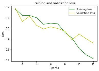
20000/20000 [==============================] - 60s 3ms/step - loss: 0.2122 - accuracy: 0.9201 - val_loss: 0.3602 - val_accuracy: 0.8666
Let’s print the loss and accuracy graphs, as the epochs increase:
#Plot the Loss
plt.clf()
loss = history.history[‘loss’]
val_loss = history.history[‘val_loss’]
epochs = range(1, len(loss) + 1)
plt.plot(epochs, loss, ‘g’, label=’Training loss’)
plt.plot(epochs, val_loss, ‘y’, label=’Validation loss’)
plt.title(‘Training and validation loss’)
plt.xlabel(‘Epochs’)
plt.ylabel(‘Loss’)
plt.legend()
plt.show()
Plot the accuracy
plt.clf()
acc = history.history[‘accuracy’]
val_acc = history.history[‘val_accuracy’]
plt.plot(epochs, acc, ‘g’, label=’Training acc’)
plt.plot(epochs, val_acc, ‘y’, label=’Validation acc’)
plt.title(‘Training and validation accuracy’)
plt.xlabel(‘Epochs’)
plt.ylabel(‘Accuracy’)
plt.legend()
plt.show()
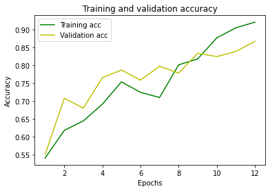
We can save the model thus obtained on the disk to use it in production during the future inference phases.
#save the model to disk
filename = ‘finalized_model_sentiment.sav’
pickle.dump(model, open(filename, ‘wb’))
We have achieved quite some high accuracy.
The moment of truth has come: let’s try to make the prediction on some test data and check if it is adequate or not!
Let’s use, for example, a review that we know is positive (in the test dataset):
#Display the review to be predicted
#0=Negative
#1=Positive
review_index = 2
y_test[review_index]
Result = 1
Let’s make the prediction by using the model built earlier:
#Sentiment Prediction
#Make the inference by using the fitted RNN model
pred = model_lstm.predict(X_test[review_index].reshape(-1,256))
print(“\n\033[1mPredicted sentiment [0=Negative – 1=Positive]: %.0f”%pred.argmax(),”\033[0m \n “)
print(“Predicted probability array:”)
print(pred)
Result:
Predicted sentiment [0=Negative - 1=Positive]: 1

Predicted probability array:
[[0.00472206 0.995278  ]]
The model predicted that the review under consideration is positive with a 99.5278% probability… What a great result!
Interested in learning more about Machine Learning and AI applications?
Here you can find a book about it:
https://www.amazon.com/dp/B08GFL6NVM
